Modern interpretation of Johanssen’s results best tackled after mastering some statistics
Intro to statistics
Completed:
Populations and samples
Measures of central tendency
Estimation of genetic and non-genetic causes for phenotypic value
Measures of dispersion and variability
Summarize certain important points we’ve just covered
Starting
Decomposing variability into causal components: Analysis of Variance (ANOVA)
Measures of shared causes: Correlation and Regression
Causal components of variance
Phenotypic variance important in evolution by natural selection
Natural selection acts only on the phenotype
Predicting evolutionary response (breeder’s equation R = h2s )
Requires knowing heritability: ratio of genetic variance to phenotypic variance
Broad-sense heritability is ratio of genotypic variance to phenotypic variance
The proportion of phenotypic variance that is not due to environmental differences
Remember that VP = VG + VE
So, could obtain VG by subtraction:
VG = VP - VE
Just need to estimate VE
Class exercise
Design experiment to estimate environmental variance (VE)
First, generate appropriate equation to estimate environmental variance
Then design experiment to obtain the necessary parameters
Discussion
First, generate appropriate equation to estimate environmental variance

Design necessary experiment
Example using one of Johanssen’s pure breeding lines
Other experiments that estimate V(E)
Nilsson-Ehle (1908)
Is there V(E)?
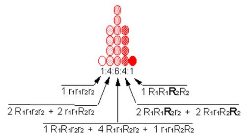
Zero V(E)
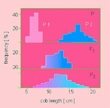
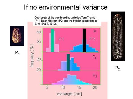
East (1910)
Is there V(E)?
What it would look like if no V(E)
Considerable V(E)
Shortcoming of our technique
Can you discern a shortcoming of the technique we’ve been exploring?
Decomposing variance into causal components
Now use analysis of variance (ANOVA) to partition the phenotypic variance into its causal components
Suppose we have five seeds from each of Johanssen’s 19 pure lines = 95 seeds
Phenotypic values
The observed population mean phenotype is:

Also called the grand mean
Phenotypic variance
Estimate the observed phenotypic variance in a population of 95 individuals by examining the deviation of each individual’s phenotype from the population mean phenotype
This is also called the total mean square = MST = (SST/dfT)
Phenotypic mean square = total mean square
The phenotypic sums of squares, then, is
Its degrees of freedom are the total experiment size (T = nm) minus 1 (used to estimate the grand mean)
In our experiment d.f. = mn-1 = (19x5)-1 = 95 – 1 = 94
Partitioning phenotypic variance
Phenotypic variance (or mean square) is composed of two causal components
Genotypic variance component
Environmental variance component
To partition phenotypic variance
Need to partition the sums of squares
Partition sums of squares by expanding around the genotype means
Here is the equation for genotypic mean

Simply
Add genotypic mean to one place on right hand side of equation
Subtract genotypic mean to another place on right had side of equation
Because adding one and subtracting one, overall effect is no change in value
What does this trick accomplish?
Produces two kinds of deviation
Within pure line environmental deviations
Deviations of individual seeds from the line mean
Among pure line genotypic deviations
Deviations of each line from the population mean
Now, do the multiplication:
Everything within the bracket can be broken up because
Summation of sums = sum of summations
Right hand side of equation now has three terms
Left hand term is sum of squares of within pure line deviations
Right hand term is sum of squares of among pure line deviations
Center term is crossproduct
Don’t need to worry about what it means because it is the product of two sums of deviations
And, what do deviations sum to?
Further, because the right hand term doesn’t include j, we can sum it over all j
To obtain
Hence, phenotypic sums of squares partitions into two components
Hence, 
Sums of squares of environmental deviations
The 1st term on the right side is the sums of squares of deviations of seeds from their pure line (genotypic) mean
Sums of squares of genotypic deviations
The 2nd term on the right side is the sums of squares of deviations of line means from the population mean (grand mean)
Partition phenotypic variance by using means squares to estimate the variance components
Estimating environmental variance
Environmental variance can be estimated by the error mean square
In our experiment, d.f. = 95 – 19 = 76
The mean square error is also an estimate of the sampling error, 
Estimating genotypic variance is somewhat more complex
Here’s the genotypic mean square
In our experiment, d.f. = 19 – 1 = 18
This value is the observed variance among line means
The observed variance among the genotype means is not the best estimate of the genotypic variance
It is biased by the sampling error of the means
The variance of observed genotypic means is a function the sum of the
variance of the true genotypic means,  , and their
sampling error,
, and their
sampling error, 
The sampling error of a mean is 
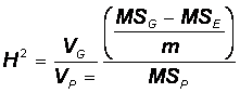
To find better estimate of genotypicvariance, go back to genotypic sums of squares
Expected genotypic sums of squares is: 
Where
![]() = variance of true genotypic means
= variance of true genotypic means
and
![]() = sampling error of
true genotypic means
= sampling error of
true genotypic means
The sampling error of a mean is ![]()
Hence, 
Factor out m : ![]()