Copyright (©) John Huelsenbeck
Do not copy without permission of author

Lecture: Phylogenetic Methods
John Huelsenbeck

Many different methods (well over 100) have been devised to estimate phylogenies. Despite the large number of methods, these methods can be grouped into three main classes: likelihood methods, distance methods, and parsimony methods. In this handout, I provide a general description of each class of methods, with examples.

Maximum Likelihood

The method of maximum likelihood was first proposed by the English statistician (and population geneticist!) R. A. Fisher. The maximum likelihood method finds that estimate of a parameter which maximizes the probability of observing the data given a specific model for the data.

A simple example of maximum likelihood estimation

As an example, consider an experiment in which a coin is flipped n times. Let heads be denoted 1, tails be denoted 0. The outcome for a particular experiment might be 0, 0, 1, 0, 1, 1, 0, 0, 0, 1. We will assume that each coin flip is distributed according to a Bernoulli distribution

,

where p is the probability of heads and x is the experimental outcome (i.e., heads or tails). Note that if p is 0.6, then f(1, 0.6) is 0.6 and f(0, 0.6) is 0.4. Many independent Bernoulli's are distributed as a binomial distribution.

We will define the likelihood function as

.

In the case of the coin flips where we are assuming a Bernoulli distribution for each flip, q = {p}. The likelihood function for the coin flips is

,

,

,

which becomes after taking the log of both sides of the equation

.

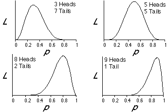
The following figures show plots of likelihood, L, as a function of p for several different possible outcomes of 10 flips of a coin. Note that for the case in which 3 heads and 7 tails were the outcome of our experiment, that the likelihood is maximized when p is 0.3. Similarly, p is 0.5 for the case of 5 heads and 5 tails, p is 0.8 for the case of 8 heads and 2 tails, and p is 0.9 for the case of 9 heads and 1 tail. The likelihood is maximized when p is the proportion of the time that heads appeared in our experiment of coin flips. This illustrates a "brute force" way to find the maximum likelihood estimate of p.

Instead of evaluating the likelihood for many values of p, we could also find the maximum likelihood estimate of p analytically. We can do this by taking the derivative of the likelihood function with respect to p and finding where the slope is 0.

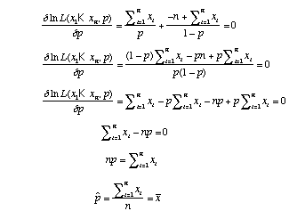
Our estimate of p (the probability of heads) is just the proportion heads that we observed in our experiment. This result is satisfying in that it makes intuitive sense.

Maximum likelihood in phylogenetics

The application of maximum likelihood estimation to the phylogeny problem was first suggested by Edwards and Cavalli-Sforza (1964). Neyman (1971) applied maximum likelihood estimation to molecular sequences using a simple model of symmetric change assuming substitutions were random and independent among sites. This model was limited to three taxa. It was not until Felsenstein (a genuine phylogenetic god) (1981) that a general maximum likelihood approach was fully developed for nucleotide sequence data. Bishop and Friday (1985) developed a maximum likelihood approach to estimate phylogenies based on amino acid sequence data which assumed constancy of evolutionary rate among lineages. Kishino et al. (1990) later extended maximum likelihood with amino acids that does not assume rate constancy among lineages, allows unequal transition probabilities, and accounts for insertion/deletion events. Below I outline the basic strategy for obtaining maximum likelihood estimates of phylogeny.

Conceptually, maximum likelihood in phylogenetics is as simple as the example given above for finding the estimate of the probability of heads in a coin-flip experiment. However, the data is usually denoted in a slightly different manner and the probability density function is more complicated.

The data for molecular phylogenetic problems are the individual site patterns. For the following aligned DNA sequences of four taxa

Taxon I ACCAGC
Taxon II AACAGC
Taxon III AACATT
Taxon IV AACATC

the observations are x1 = (A, A, A, A)T, x2 = (C, A, A, A)T, x3 = (C, C, C, C)T, x4 = (A, A, A, A)T, x5 = (G, G, T, T)T, and x6 = (C, C, T, C)T, where the superscript "T" means the transpose of the vector. In other words, our sample consists of n vectors (as many vectors as there are sites in the sequence, with the elements of each vector denoting the nucleotide state for each taxon for site i.

Now that we understand how the data are denoted, how do we calculate the probability of observing some xi?. To do this, we must explicitly describe our model of evolution. In phylogenetics, a model consists of three parts: a tree, branch lengths on this tree, and a model of DNA substitution.

Let's calculate the probability for just one of the nucleotide sites, above (x5), for the following tree (with branch lengths assigned; the bi's).

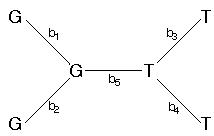
Also, we will assume a very simple model of DNA substitution (called the Jukes-Cantor model). The probability of a change under the Jukes-Cantor model is

,

where b is the length of the branch (in terms of number of substitutions per site) and a change to each nucleotide is equally probable. The probability of no change PNC(bi) is just 1 PC(bi).

For the time being, let's assume that the nucleotide sites at the internal nodes are also known. The probability for site 5 is just the probability of no change along branch 1 times the probability of no change along branch 2 times the probability of no change along branch 3 times the probability of no change along branch 4 times the probability of a change from a G to a T along branch 5.

.

Here, Q is a vector containing all of the branch lengths. Of course, with real sequence data, we do not know the states of the internal branches. What we have to do then is sum our probabilities over all possible assignments of states to the internal nodes. In the example above, the probability of site 5 would be a sum of 16 terms.

The likelihood of the tree is

.

Our goal is to visit each possible bifurcating tree in turn. For each tree, we find that combination of branch lengths which maximize the likelihood of the tree (which maximizes the likelihood function, above). Our maximum likelihood estimate of phylogeny is the tree with the greatest likelihood.

This all takes a lot of time. Fortunately, there are a lot of short cuts that can be taken. For example, Felsenstein described a method that avoids summing over all possible assignments of states to the internal branches. There are also nifty ways of optimizing branch lengths that entail taking the first and second derivatives of the likelihood function with respect to the branch of interest. Finally, in practice we can avoid visiting each possible tree and concentrate on those that have a good chance of maximizing the likelihood function.

Distance Methods

Distance methods estimate trees in a two step process. First, pairwise comparisons of all sequences are made and a distance matrix is produced. Then some optimality criterion uses this distance matrix to estimate a tree. As an example of a distance method, I will discuss the minimum evolution criterion.

Minimum Evolution

Minimum evolution is a distance method described by Cavalli-Sforza and Edwards (1967), Kidd and Sgaramella-Zonta (1971), and Rzhetsky and Nei (1992).

Again, lets consider the following sequences

Taxon I ACCAGC
Taxon II AACAGC
Taxon III AACATT
Taxon IV AACATC

From these sequences, we can come up with a matrix of pairwise comparisons. If we compare the sequences for taxa I and II, we find that there is one change out of six sites. The distance between these two taxa is then 1/6 (note: there are a lot of transformation we could impose that would correct for multiple substitutions, but I don't want to get into that). The full distance matrix would be

I'll denote the elements of the matrix d1 to d6

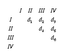
Minimum evolution picks that tree which minimizes the sum of the lengths of the branches:

.

How are the bi's calculated with minimum evolution? Consider the following tree

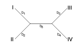
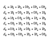
We can write our observed di's in terms of the bi's of this tree. For example, the distance between taxa I and II (d1) is the sum of b1 and b2. In general, we can write a system of equations for all six of the di's:

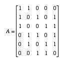
We can also write this system of equations in matrix form. First, all of the 1's and 0's go into the adjacency matrix, A.

The di's go into a vector d and the bi's go into a vector b. The system of equations is then

.

The least squares estimate of b is given by

,

where "T" denotes the transpose and "1" denotes the inverse of the matrix A. Now we have finished all of the difficult work. It is a simple manner to sum the elements of the vector b for our tree. It is not so simple, however, to visit all possible trees to find that tree which minimizes this sum. Fortunately, we can take short cuts by visiting only those trees which are likely to minimize the sum of the branch lengths. Also, there are short cuts to the matrix operations that I described above (this was the novel part of the Rzhetsky and Nei, 1992 paper). Furthermore, the neighbor joining algorithm is often a computationally efficient method for finding the minimum evolution tree.

Parsimony methods

The criterion for the parsimony method is identical to the criterion for the minimum evolution method! We simply sum the reconstructed changes along the branches of the tree and pick that tree with the minimum number of reconstructed changes.

We do this for all possible trees and find that tree which minimizes the total number of reconstructed changes. This tree is our best estimate of phylogeny. Of course, instead of calling this tree the minimum evolution tree we call it the maximum parsimony tree (why minimize when you can maximize!).

Unordered characters.

How does the parsimony method reconstruct the changes along the branches of the tree? One commonly used method assumes that character state transitions are unordered (Fitch, 1971). Consider the following tree with the assignments of G's and T's to the tips

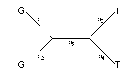
This tree can be arbitrarily rooted. I'll root it along branch 5.

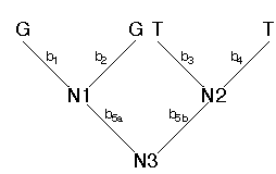
We pass down the tree and visit each node in succession (N1, N2, and then N3). For each node we visit, we examine the states assigned to the nodes above (to the left and right). For example, for N1, the states assigned to the nodes above are G and G. We can consider the assignments of states to the left and right of the node as sets of character states. In this case the set of states assigned to the left is L = {G} and the set of states assigned to the right is R = {G}. If the intersection of the sets L and R is not empty, we assign the intersection to N1. If the intersection is empty, then we assign the union of the sets to N1. Because the intersection of L and R is not empty, we assign N1 state G (N1 = {G}). Using this same procedure we would assign N2 the state T (N2 = {T}). Finally, we visit node N3. The following states are assigned to the left and to the right for N3: L = {G} and R = {T}. Because the intersection is empty, we assign the union of L and R to N3 (N3 = {G,T}). Each time the intersection of the sets to the left and to the right is empty implies one character step. For the example, above, we find that the character pattern GGTT implies one character change. We could then figure out along which branches the change occurred. However, for the parsimony criterion, we don't have to know where the change occurred, just how many occurred for that character pattern. We sum the number of changes over all sites. The result is the total length of the tree (in terms of character changes). Our job is then to find that tree with the minimum number of total changes. This tree is the maximum parsimony estimate of phylogeny. ÿ